Trying out jupyter notebook markdown generator in Jekyll
import numpy as np
import matplotlib.pyplot as plt
import scipy.io as sio
def plot_info(tit,x,y,leg=''):
    plt.title(tit)
    plt.xlabel(x)
    plt.ylabel(y)
    if leg != '':
        plt.legend(leg)
a) reading data and checking sizes
data = sio.loadmat("data.mat")
x = data.get("x")
y = data.get("y")
u = data.get("u")
v = data.get("v")
xit = np.transpose(data.get("xit"))
yit = np.transpose(data.get("yit"))
x
array([[ 0. ,  0.5,  1. , ..., 95.5, 96. , 96.5],
       [ 0. ,  0.5,  1. , ..., 95.5, 96. , 96.5],
       [ 0. ,  0.5,  1. , ..., 95.5, 96. , 96.5],
       ...,
       [ 0. ,  0.5,  1. , ..., 95.5, 96. , 96.5],
       [ 0. ,  0.5,  1. , ..., 95.5, 96. , 96.5],
       [ 0. ,  0.5,  1. , ..., 95.5, 96. , 96.5]])
y
array([[-50. , -50. , -50. , ..., -50. , -50. , -50. ],
       [-49.5, -49.5, -49.5, ..., -49.5, -49.5, -49.5],
       [-49. , -49. , -49. , ..., -49. , -49. , -49. ],
       ...,
       [ 49. ,  49. ,  49. , ...,  49. ,  49. ,  49. ],
       [ 49.5,  49.5,  49.5, ...,  49.5,  49.5,  49.5],
       [ 50. ,  50. ,  50. , ...,  50. ,  50. ,  50. ]])
np.shape(x)
(201, 194)
np.shape(y)
(201, 194)
np.shape(u)
(201, 194)
np.shape(v)
(201, 194)
- We have correct spacing, 0.5 mm
- y represents the whole diameter of the tube
- the shapes are right, i.e the rows and columns have correct sizes
b) contour of velocity field
total_velocity = np.sqrt(u**2 + v**2);

N = 20 # number of different contours
max_water = 400 # max water velocity in mm/s
max_air = 4000

# first show details in water by restricting which values are shown in the contour
# i.e specifying levels.

levels_water = np.linspace(0,max_water,N)
plt.contourf(x,y,total_velocity,levels_water)
plot_info('velocity distribution water','X','Y')
plt.colorbar()
plt.plot(xit,yit,'k',linewidth = 4)
plt.show()

levels_air = np.linspace(max_water,max_air,N)
plt.contourf(x,y,total_velocity,levels_air)
plot_info('velocity distribution air','X','Y')
plt.colorbar()
plt.plot(xit,yit,'k',linewidth = 4)
plt.show()
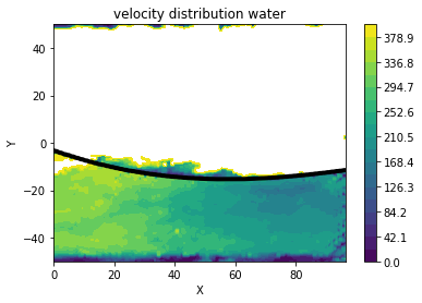
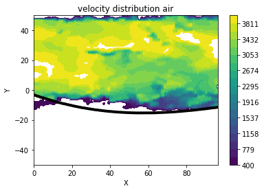
conclusions
- the water velocity is significantly lower than air velocity
- water velocity is higher at the left part of the image
- lower parts of the water are almost not moving
- one can almost observe the interface between water and air, solely from the velocity distribution
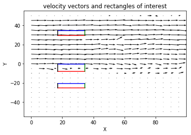
c) quiver and rectangles plot
# take a list of rectangles specified by two points, i.e two lists
# with coordinates, whose line segment is the diagonal of the rectangle
def draw_rectangles(rectangles):

    for rec in rectangles:
        point1,point2 = rec
        x1,y1 = point1
        x2,y2 = point2
        plt.plot([x1,x2],[y1,y1],'r',[x1,x2],[y2,y2],'b',[x2,x2],[y1,y2],'g',[x1,x1],[y1,y2],'k')

def downsample(A,samplerate):
    return A[::samplerate,::samplerate]

N = 10 # sample rate
x_downsampled = downsample(x,N)
y_downsampled = downsample(y,N)
u_downsampled = downsample(u,N)
v_downsampled = downsample(v,N)


# all x values equal for rectangles
x1 = 34
x2 = 69
rec_names = ['top','middle','bottom'] # used in print-outs

# indexes of rectangles on grid
rec1_index = [[34,159],[69,169]]
rec2_index = [[34,84],[69,99]]
rec3_index = [[34,49],[69,59]]

# absolute rectangle positions on grid
rec1 = [[x[1,x1],y[159,1]],[x[1,x2],y[169,1]]] # air
rec2 = [[x[1,x1],y[84,1]], [x[1,x2],y[99,1]]]  # middle air
rec3 = [[x[1,x1],y[49,1]], [x[1,x2],y[59,1]]]   # water

recs = [rec1,rec2,rec3] # rectangles to draw

draw_rectangles(recs)

plt.quiver(x_downsampled,y_downsampled,u_downsampled,v_downsampled)
plot_info('velocity vectors and rectangles of interest','X','Y')
plt.show()
d) divergence of vector field
divergence is the flux into a volume
\[\nabla \cdot \vec{v} = \frac{\partial u}{\partial x} + \frac{\partial v}{\partial y} + \frac{\partial w}{\partial z}\]The gas is incompressible, for the divergence, this means that its absolute value has to be zero
\[\frac{\partial u}{\partial x} + \frac{\partial v}{\partial y} + \frac{\partial w}{\partial z} = 0\] \[\frac{\partial u}{\partial x} + \frac{\partial v}{\partial y} = -\frac{\partial w}{\partial z}\]The sum of the acceleration for the u and v components are thus the negative of the acceleration in the w component. The reason that the code does not compute the real divergence is because we do not take the w-component into account
above I use the gradient operator to solve the problem:
\(\nabla u = \left[\frac{\partial u}{\partial x},\frac{\partial u}{\partial y} , \frac{\partial u}{\partial z} \right ]\) \(\nabla u = \left[\frac{\partial v}{\partial x},\frac{\partial v}{\partial y} , \frac{\partial v}{\partial z} \right ]\)
The components of the above equations contains what we need to compute the divergence.
dudx,dudy = np.gradient(u,0.5)
dvdx,dvdy = np.gradient(v,0.5)

div = np.sum([dudx,dvdy],axis=0);

plt.contourf(x,y,div);


plt.plot(xit,yit,'k')

draw_rectangles(recs)

plt.colorbar()
plot_info('divergence','X','Y')
plt.show()
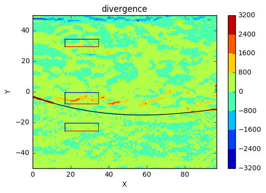
conclusions
- the divergence is high in the middle, that makes sense, since a wavefront is rushing towards the area
- other areas has low divergence, not much net volume rusing into area
- from the plot, one can conclude that the fluids are incompressible under the current environment
e) curl z-component
to get the component of curl normal to the xy-plane:
\[\gamma = \nabla \vec{v}\]$\gamma$ contains a list of the list containing the partial derivatives for each component.
\[\gamma(1)(1) = \frac{\partial u}{\partial x}, \gamma(2)(2) = \frac{\partial v}{\partial y}\]The difference of the second from the first gives us the result we want.
\[(\frac{\partial v}{\partial x}-\frac{\partial u}{\partial y})\vec(k)\]We have the necessary variables dvdx and dudy from the previous exercise
z_curl_component = dvdx - dudy

min_curl = -1500
max_curl = 4000
levels = np.linspace(min_curl,max_curl,50)
plt.contourf(x,y,z_curl_component,levels)
plt.colorbar()
plt.plot(xit,yit,'k')
plot_info('z curl component','X','Y')


draw_rectangles(recs)


plt.show()
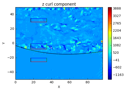
conclusions
main take-away is again that there is something intersting happening where the wavefront is headed.
f) Stokes theorm and direct circulation calculation
to take the curve integral, we can do the following $\int_\lambda \vec{v} \cdot d\vec{r}$
since we have a constant spacing in the grid of 5mm, we can calculate the curve integral for each side numerically as follows:
\(r_1 = \sum_{i=1}^{N} u(y_0,x_i)*0.5\) \(r_2 = \sum_{i=1}^{N} u(y_i,x_0)*0.5\) \(r_3 = \sum_{i=1}^{N} u(y_1,x_i)*-0.5\) \(r_4 = \sum_{i=1}^{N} u(y_i,x_1)*-0.5\)
where $x_i$ is the points in the rectangle grid in x-direction, and $x_0$ and $x_1$ etc. are constant levels that are not changing because we are doing summations vertically or horizontally in the grid, thus either x or y is constant.
stokes theorem tells us that there is a relation between the line integral and the area-integral:
$\int_\lambda \vec{v} \cdot d\vec{r} = \int_\sigma \nabla \times \vec{v} \cdot \vec{n} \quad d\sigma$
where $\times$ is the cross product operator:
\[\vec{a} \times \vec{b} = \quad \left| \begin{matrix} \vec{i} & \vec{j} & \vec{k} \\ a_i & a_j & a_k \\ b_i & b_j & b_k \end{matrix}\right|\]and $\nabla$ is:
\[\nabla = \left [\frac{\partial}{\partial x},\frac{\partial}{\partial y},\frac{\partial}{\partial z} \right]\]Our area is $0.25mm^2$, since the cells in the grid are squares with $s=0.5$
we have the z-component of the curl from previous exercise. The curl is different for each cell in our grid.
calculation is done with a sum as the direct calculation over
def get_circulation(point1,point2,u,v):
    spacing = 0.5 # grid spacing in mm
    x1,y1 = point1
    x2,y2 = point2

    # circulation around horizontal lines of rectangle
    r1 = np.sum(u[y1,x1:x2] * (spacing));
    r3 = np.sum(u[y2,x1:x2] * -(spacing));

    # for the vertical lines of the rectangle, the column are constant and rows
    # are changing
    r2 = np.sum(v[y1:y2,x1] * spacing);
    r4 = np.sum(v[y1:y2,x2] * -spacing);

    total_circulation = r1 + r2 + r3 + r4;

    print('x1 = %.2f \ny1 = %.2f \nx2 = %.2f \ny2 = %.2f\n' % (x1,y1,x2,y2));
    print('r1 = %.2f \nr2 = %.2f \nr3 = %.2f \nr4 = %.2f\n' % (r1,r2,r3,r4));
    print('\n\n total_circulation %.2f \n\n'% total_circulation);

    return total_circulation


def new_grid(A,point1,point2):
    x1,y1 = point1
    x2,y2 = point2
    return A[y1:y2,x1:x2]
#calculate circulation
circ_direct_air = get_circulation(*rec1_index,u,v)
circ_direct_middle = get_circulation(*rec2_index,u,v)
circ_direct_water = get_circulation(*rec3_index,u,v)
circ_direct = [circ_direct_air,circ_direct_middle,circ_direct_water]

# using stokes

spacing = 0.5
area_cell = spacing**2;
z_curl_component_scaled = z_curl_component*area_cell;

# we have to cut out relevant sub-grids based on rectangles
z_curl_component_scaled_rec1 = new_grid(z_curl_component_scaled,*rec1_index);
z_curl_component_scaled_rec2 = new_grid(z_curl_component_scaled,*rec2_index);
z_curl_component_scaled_rec3 = new_grid(z_curl_component_scaled,*rec3_index);

# sum all rows and columns
circ_stokes_air = np.sum(z_curl_component_scaled_rec1);
circ_stokes_middle = np.sum(z_curl_component_scaled_rec2);
circ_stokes_water = np.sum(z_curl_component_scaled_rec3);
circ_stokes = [circ_stokes_air,circ_stokes_middle,circ_stokes_water]
x1 = 34.00
y1 = 159.00
x2 = 69.00
y2 = 169.00

r1 = 68091.84
r2 = -632.84
r3 = -66448.39
r4 = -235.16


 total_circulation 775.45


x1 = 34.00
y1 = 84.00
x2 = 69.00
y2 = 99.00

r1 = 113.52
r2 = 236.40
r3 = -59592.74
r4 = -462.29


 total_circulation -59705.11


x1 = 34.00
y1 = 49.00
x2 = 69.00
y2 = 59.00

r1 = 5000.81
r2 = -70.26
r3 = -5270.32
r4 = -185.42


 total_circulation -525.18
# Results

print("\n direct calculations\n")
for rec_name,c in zip(rec_names,circ_direct):
    print("circulation of %s rectangle: %.2f " % (rec_name,c))

print("\n calculations with stokes\n")
for rec_name,c in zip(rec_names,circ_stokes):
    print("circulation of %s rectangle: %.2f " % (rec_name,c))
 direct calculations

circulation of top rectangle: 775.45
circulation of middle rectangle: -59705.11
circulation of bottom rectangle: -525.18

 calculations with stokes

circulation of top rectangle: -1401.85
circulation of middle rectangle: -13011.09
circulation of bottom rectangle: 278.21
conclusions
- There is greater circulation around the middle rectangle, which is consistent with the velocity field
- the high z-components of the curl in previous exercises hinted to high circulation around middle area. Confirmed.
- low circulations around other rectangles as expected
g ) Gauss’s theorm
calculation of flux through the sides of the rectangle is similar numerically to the circulation, only that u and v are interchanged for each side. example: the flux through r2(green) is decided by u and not v like in the circulation calculation
gauss theorem is a relation between area and volume integrals
\[\int_\sigma \mathbf{v} d\sigma = \int_V \nabla \cdot \mathbf{v}dV\]numerically, the calculation is similar to the above examples.
def get_flux(point1,point2,u,v):
    spacing = 0.5 # grid spacing in mm
    x1,y1 = point1
    x2,y2 = point2

    # circulation around horizontal lines of rectangle
    r1 = np.sum(v[y1,x1:x2] * (spacing));
    r3 = sum(v[y2,x1:x2] * -(spacing));

    # for the vertical lines of the rectangle, the column are constant and rows
    # are changing
    r2 = sum(u[y1:y2,x1] * spacing);
    r4 = sum(u[y1:y2,x2] * -spacing);

    total_flux = r1 + r2 + r3 + r4;

    print('x1 = %.2f \ny1 = %.2f \nx2 = %.2f \ny2 = %.2f\n' % (x1,y1,x2,y2));
    print('r1 = %.2f \nr2 = %.2f \nr3 = %.2f \nr4 = %.2f\n' % (r1,r2,r3,r4));
    print('\n\n total flux %.2f \n\n'% total_flux);

    return total_flux
# direct calculation

flux_direct_air = get_flux(*rec1_index,u,v)
flux_direct_middle = get_flux(*rec2_index,u,v)
flux_direct_water = get_flux(*rec3_index,u,v)
fluxes_direct = [flux_direct_air,flux_direct_middle,flux_direct_water]

# using green's theorem

# we have div = divergence from previous exercise
div_scaled = div * area_cell; # area is equal in each grid_cell

div_rec1 = new_grid(div_scaled,*rec1_index);
div_rec2 = new_grid(div_scaled,*rec2_index);
div_rec3 = new_grid(div_scaled,*rec3_index);

flux_gauss_air = np.sum(np.sum(div_rec1));
flux_gauss_middle = np.sum(np.sum(div_rec2));
flux_gauss_water = np.sum(np.sum(div_rec3));
fluxes = [flux_gauss_air,flux_gauss_middle,flux_gauss_water]
x1 = 34.00
y1 = 159.00
x2 = 69.00
y2 = 169.00

r1 = -1576.77
r2 = 19172.62
r3 = 2090.79
r4 = -19780.11


 total flux -93.46


x1 = 34.00
y1 = 84.00
x2 = 69.00
y2 = 99.00

r1 = 5005.85
r2 = 10237.07
r3 = 3911.98
r4 = -13131.81


 total flux 6023.08


x1 = 34.00
y1 = 49.00
x2 = 69.00
y2 = 59.00

r1 = 183.80
r2 = 1590.82
r3 = -262.45
r4 = -1397.10


 total flux 115.07
# Results

print("\n direct calculations\n")
for rec_name,flux in zip(rec_names,fluxes_direct):
    print("flux of %s rectangle: %.2f " % (rec_name,flux))

print("\n calculations with stokes\n")
for rec_name,flux in zip(rec_names,fluxes):
    print("flux of %s rectangle: %.2f " % (rec_name,flux))
 direct calculations

flux of top rectangle: -93.46
flux of middle rectangle: 6023.08
flux of bottom rectangle: 115.07

 calculations with stokes

flux of top rectangle: -852.32
flux of middle rectangle: 59614.87
flux of bottom rectangle: 529.03
conclusions
- high flux into middle rectangle makes sense, since the wavefront is heading into the area.